How to fit a manifold?

This is a quick introduction of manifold fitting. A PDF version is also available. More details can be found in:

• Fefferman, C., Ivanov, S., Kurylev, Y., Lassas, M., & Narayanan, H. (2018, July). Fitting a putative manifold to noisy data. In Conference On Learning Theory (pp. 688-720). PMLR.
• Yao, Z., & Xia, Y. (2019). Manifold fitting under unbounded noise. arXiv preprint arXiv:1909.10228.
• Yao, Z., Su, J., Li, B., & Yau, S. T. (2023). Manifold fitting. arXiv preprint arXiv:2304.07680.

Method

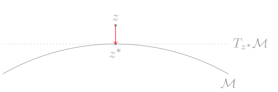
Let $z$ be the point of interest, which is close to $\mathcal{M}$, and $z^{\ast }=\arg \underset{z^{\prime }\in \mathcal{M}}{min}d(z^{\prime },z)$ be the projection of $z$ on $\mathcal{M}$. Intuitively, the estimation of manifold can be viewed as ‘‘pushing’’ $z$ to $z^{\ast }$.

This pushing process involves two key components: direction and distance. The direction should be perpendicular to $T_{z\ast }\mathcal{M}$, which can be deduced from the local ‘‘covariance’’ structure, while the distance $d(z,\mathcal{M})$ might be estimated using the local average. The following subsections will introduce some intuitive concepts related to this process. For more details, please refer to the papers mentioned previously.

Estimate Direction from Local ‘‘Covariance’’

For each point $y_i\in {\mathcal{Y}}_N$, let $y_i^{\ast }$ be its projection on $\mathcal{M}$. Assume the normal space of $\mathcal{M}$ at $y_i^{\ast }$ has orthonormal basis $\{u_1,\dots ,u_{D-d}\}$, we use

$${\mathrm{\Pi }}_{y_i^{\ast }}^{\perp }=(u_1,\dots ,u_{D-d})(u_1,\dots ,u_{D-d}{)}^{\mathrm{\top }}=\sum _{k=1}^{D-d}{u}_k{u}_k^{\mathrm{\top }}$$

to represent the projection matrix onto this space. This projection matrix can be estimated from the local variation centered at $y_i$, and the estimator of ${\mathrm{\Pi }}_{y_i^{\ast }}^{\perp }$ is denoted as ${\hat{\mathrm{\Pi }}}_{y_i}^{\perp }$.

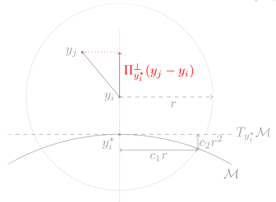
Let ${\mathcal{B}}_D(y_i,r)$ be the $D$-dimensional Euclidean ball centered at $y_i$ with radius $r$. If $r$ is ‘‘large’’ enough, such that $\Vert y_i-y_i^{\ast }\Vert \le \Vert {\xi }_i\Vert \le c_{0}r$, the area of ${\mathcal{B}}_D(y_i,r)\cap \mathcal{M}$ roughly has radius $c_{1}r$, and the variation of $\mathcal{M}$ along the normal direction is less than $c_2{r}^2$ due to the reach. Then, since the distribution of $X$ is smooth, the variation of $Y-y_i$ along direction:

• $\leftrightarrow$: is roughly in the order of $(c_{1}r{)}^2+{\sigma }^2$;
• $\updownarrow$: is roughly bounded above by the order of $(c_2{r}^2{)}^2+{\sigma }^2$.

Thus, we can define

$${\hat{\mathrm{\Sigma }}}_{r,i}=\frac{\sum _{j=1}^N(y_j-y_i)(y_j-y_i{)}^{\mathrm{\top }}\mathbb{I}(\Vert y_j-y_i\Vert \le r)}{\sum _{j=1}^n\mathbb{I}(\Vert y_j-y_i\Vert \le r)}.$$

Then perform SVD on ${\hat{\mathrm{\Sigma }}}_{r,i}$ to obtain $\{{\lambda }_1<\cdots <{\lambda }_D\}$ and $\{v_1,\dots ,v_D\}$, and estimate ${\mathrm{\Pi }}_{y_i^{\ast }}^{\perp }$ with ${\hat{\mathrm{\Pi }}}_{y_i}^{\perp }=(v_1,\dots ,v_{D-d})(v_1,\dots ,v_{D-d}{)}^{\mathrm{\top }}=\sum _{k=1}^{D-d}{v}_k{v}_k^{\mathrm{\top }},$ whose estimation error can be bounded.

Smoothing System

To make the overall estimation smooth enough, the weight function for $y_i$ with respect to $z$ is defined as

$${\tilde{\alpha }}_i(z)={(1-\frac{\Vert z-y_i{\Vert }^2}{r^{\prime 2}})}^{\beta }\mathbb{I}(\Vert z-y_i\Vert \le r^{\prime }),{\alpha }_i(z)=\frac{{\tilde{\alpha }}_i(z)}{\sum _{i=1}^n{\tilde{\alpha }}_i(z)},$$

where $\beta \ge 2$ is a parameter corresponding to the smoothness. Then, for $z$, a smooth reference point can be given by ${\hat{\mu }}_z=\sum _{i=1}^N{\alpha }_i(z)y_i$, and a smooth projection matrix is calculated as

$${\mathrm{\Psi }}_z={\mathbb{P}}_{D-d}(\sum _{i=1}^N{\alpha }_i(z){\hat{\mathrm{\Pi }}}_{y_i}^{\perp }),$$

where ${\mathbb{P}}_k(A)$ stands for the projection of matrix $A$ onto the span space corresponding to its largest $k$ eigenvalues.

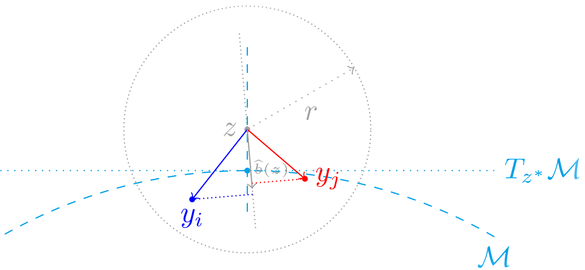
The Manifold Estimator

The vector from $z^{\ast }$ to $z$ can be estimated with the bias vector

$$\hat{b}(z)=\sum _{i=1}^n{\alpha }_i(z){\mathrm{\Psi }}_z(z-y_i)={\mathrm{\Psi }}_z(z-{\hat{\mu }}_z),$$

which can be shown

• $\Vert \hat{b}(z)\Vert$ close to $\Vert z-z^{\ast }\Vert$;
• Jacobian matrix of $\hat{b}(z)$ is close to ${\mathrm{\Phi }}_z$, i.e. $\Vert J_b(z)-{\mathrm{\Psi }}_z\Vert \le C\sigma /r^{\prime }+o_p(1)$;
• Hessian matrix of $\hat{b}(z)$ is lower bounded.

Finally, the manifold estimator is given by

$$\hat{\mathcal{M}}=\{z\in {\mathbb{R}}^D:d(z,\mathcal{M})<c{r}^{\prime },\hat{b}(z)=0\}.$$

Under all the error bounds and all the smoothness, for any $z^{\prime }\in \hat{\mathcal{M}}$, with high probability,

• $z^{\prime }$ is close to $\mathcal{M}$;
• in its neighborhood, $\hat{b}(z)$ is rank $D-d$.

Hence, with high probability, $\hat{\mathcal{M}}$ is a $d$-dimension manifold, close to $\mathcal{M}$, and its reach can be bounded via the Hessian of $\hat{b}(z)$.